Not All Field Goals Weigh the Same

With 7:33 remaining in the third quarter, the Houston Texans faced fourth-and-one at the Cincinnati 40-yard line. Houston trailed 10-3 and had managed only a field goal through more than two quarters of football. Head coach DeMeco Ryans had three choices. He could punt and give Cincinnati possession, keep his offense on the field and attempt to gain one yard, or send Ka’imi Fairbairn out to attempt a 58-yard field goal. Each option carried uncertainty, and each would leave Houston in a different position depending on the outcome.¹

There was good reason to trust Fairbairn. One week earlier, Houston had faced fourth-and-four at the Buffalo 39-yard line with approximately seven minutes remaining in the fourth quarter. The Texans trailed 30-28 when Fairbairn made a 58-yard field goal to give Houston the lead.² When Ryans later explained his decision against Cincinnati, he pointed to that earlier kick.³ Fairbairn had made one from essentially the same spot the previous week, and Houston trusted him to do it again.

The reasoning is familiar because we make decisions this way all the time. A product launch succeeds, so management becomes more confident in the next launch. An investment performs well, so additional capital flows toward the same strategy. Previous results are useful information, and good decision-makers should update their expectations when new evidence becomes available. The difficulty is determining how much weight that evidence deserves, particularly when the most recent outcome is memorable.

Fairbairn had made nine of thirteen field-goal attempts from 50 yards or longer during the previous regular season.⁴ All thirteen were between 50 and 57 yards, so the record did not directly establish his probability of making a 58-yard attempt. Our distance-based model, which incorporated the closed-roof environment but did not depend on Fairbairn’s individual record, estimated approximately a 67 percent chance of success. Alternative estimates incorporating his kicking history were similar, ranging from roughly 67 to 69 percent.⁵

That is a respectable probability for a long field goal, but it is far from a guarantee. Weather forecasting provides a useful comparison. If a well-calibrated forecast assigns a 70 percent chance of rain, rain should occur on approximately seven of every ten comparable forecasts. On the other three occasions, it should remain dry. We would not conclude that the forecast was wrong simply because one of those dry days occurred. The forecast never promised rain. It described the likelihood of an uncertain event.

The same reasoning applies to Houston’s alternative. Earlier in the Cincinnati game, with the score tied 0-0, the Texans faced fourth-and-one at the Cincinnati 18. Houston went for it, and David Montgomery was stopped for a one-yard loss. Just before the later fourth-down decision, Houston had also failed to convert a third-and-one. Yet Houston had converted two fourth-and-one rushing attempts the previous week.⁶ The recent evidence was mixed, and a few outcomes could not establish that the offense had suddenly lost its ability to gain a yard.

In Thinking in Bets, Annie Duke describes the tendency to evaluate decisions by their outcomes as “resulting.”⁷ Recent events can become disproportionately influential because they are easier to remember. Houston had evidence that Fairbairn could make a 58-yard field goal and evidence that its offense could fail to gain one yard. Neither observation was irrelevant, but neither was sufficient to determine which alternative offered the better opportunity. To evaluate that choice, we need to consider not only the probability of success, but also what success actually provides.

What Does Success Buy?

Fairbairn’s attempt against Cincinnati eventually came up short. If we begin our evaluation with the miss, hindsight immediately becomes part of the analysis. Houston attempted a difficult field goal, failed to score, and surrendered possession. It becomes tempting to criticize the choice because we already know the outcome. Ryans did not have that information when he made the decision, so we should evaluate the alternatives without relying on it.

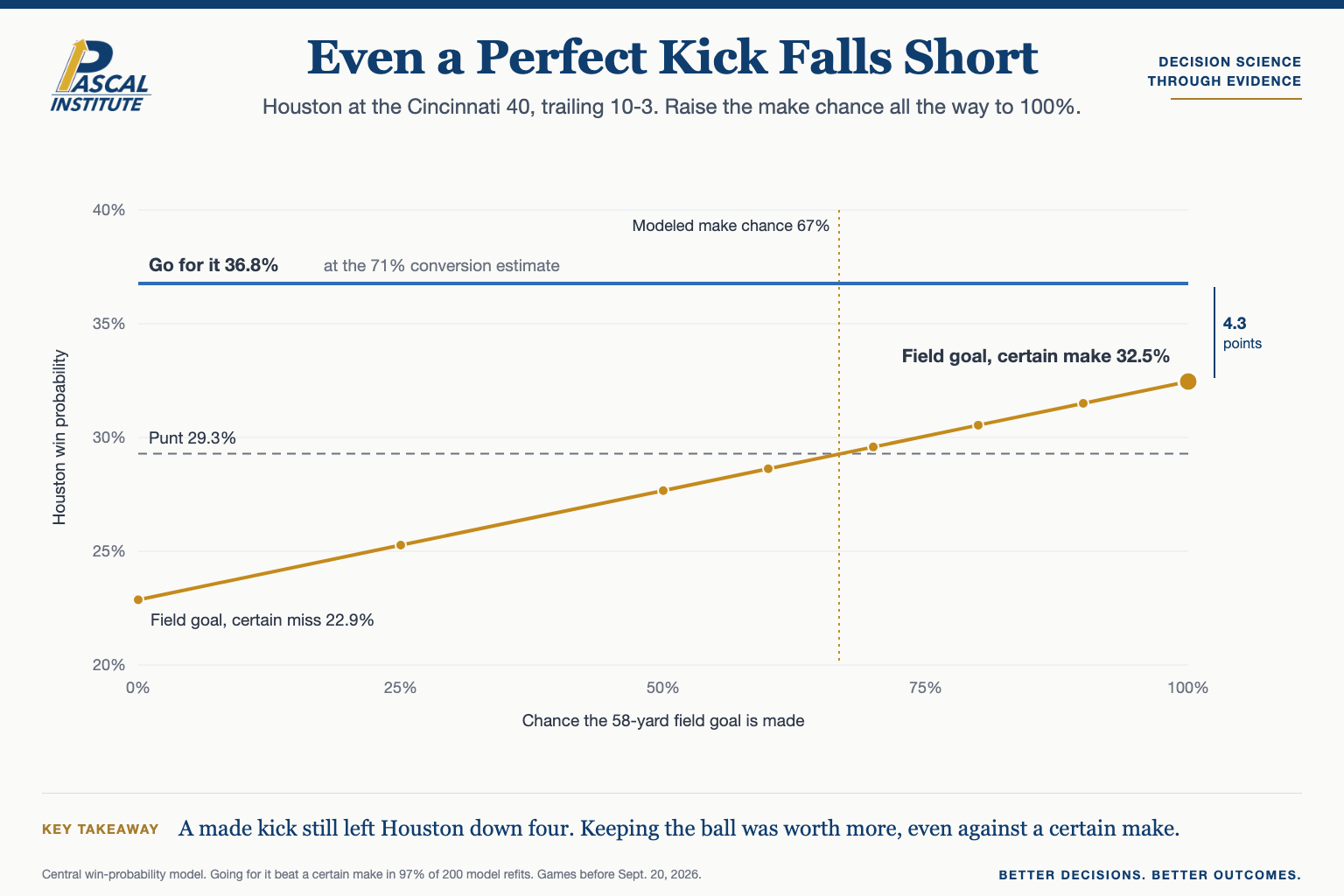
We can remove the temptation by giving Houston the result it wanted. Assume Fairbairn makes the kick. The score changes from 10-3 to 10-6, and the Texans have three additional points. They still trail by four, however, and still need a touchdown to take the lead. The field goal improves the scoreboard without changing the basic requirement for Houston to move ahead.

Win probability is the share of games a team goes on to win from a given situation, and it is how we compare the three choices. Our model estimated Houston’s win probability after a successful field goal at approximately 32.5 percent. That number is useful only when compared with the alternatives. At the estimated conversion probability, going for fourth-and-one produced a modeled win probability of approximately 36.8 percent. Even when we assume Fairbairn makes the field goal with certainty, the central model still favors going for it. That comparison also survived 97 percent of the win-probability model refits we examined.⁸

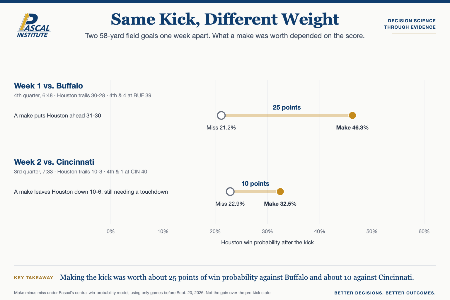
The previous week’s kick against Buffalo had a different value. Making that field goal instead of missing it represented an estimated swing of approximately 25 percentage points of win probability. Against Cincinnati, the corresponding make-versus-miss difference was approximately ten percentage points. These comparisons measure the difference between the successful and unsuccessful field-goal outcomes in each game, not the improvement relative to the pre-decision state.⁸

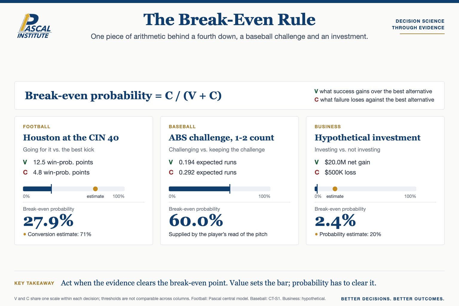
Our model estimated Houston’s probability of converting fourth-and-one at approximately 71 percent. Given the estimated values of the alternatives, the central model placed the break-even conversion probability near 28 percent. That threshold incorporated a modeled field-goal make probability of approximately 67 percent. We repeatedly refit the win-probability model using different samples of historical games. The threshold moved between about 18 and 48 percent across refits, but at the estimated conversion probability, going for it remained preferred in every one.⁸

That conclusion does not mean the Texans would have converted. Nor does it suggest that Fairbairn was incapable of making the kick. The evidence available at the time favored attempting to gain one yard because the expected value of retaining possession exceeded the value of the field-goal alternative. We can reach a defensible decision without knowing what will happen next. Probability matters, but probability alone does not determine whether an opportunity is worth pursuing.

Putting a Value on Opportunity

We encountered the same problem during our research into Major League Baseball’s ABS Challenge System. A player who believes an umpire incorrectly called a pitch must decide whether to use one of the team’s limited challenges. The probability that the player is correct matters, but it cannot answer the question by itself. Correcting one call may produce a modest improvement in the count, while correcting another may prevent a strikeout. An unsuccessful challenge also consumes a resource that could be valuable later in the game.

Our research led to Challenge Threshold, a reference measure designed to estimate the confidence required for a challenge to break even. Under our CT-S1 model, V is the immediate expected-run gain from correcting an incorrect call and C is the modeled future expected-run value of preserving the challenge. Both are measured in expected runs. Under the fixed-path assumption, holding the subsequent game path fixed outside the inventory effect, the relationship becomes:

Decision Opportunity Score, or DOS, expresses the other side of that relationship:

Challenge Threshold describes how confident the player would need to be for the opportunity to break even under the named model. DOS expresses the relative value of the immediate opportunity compared with preserving the challenge. DOS is not a probability, an estimate of player confidence, or a recommendation. Its value depends on the model’s assumptions, and alternative defensible conventions can produce materially different thresholds.

Consider two states from that research. In both, the modeled future value of preserving a challenge was 0.292 expected runs. Correcting the call in a 1-1 count produced an immediate modeled value of 0.142 expected runs, while the corresponding value in a 1-2 count was 0.194. Under the named reference, the higher correction value lowered the confidence required for break-even. Nothing implied that the player became better at recognizing an incorrect call. The circumstances changed the value of being right.⁹

The baseball formula should not be applied unchanged to football or business. Nevertheless, the underlying break-even logic is more general. In a simplified decision where success produces an incremental gain V and failure an incremental loss C relative to an alternative, the break-even probability is C divided by V plus C. Both must be measured on a compatible value scale, and additional outcomes or continuation effects require a more complete model. Houston’s analysis used football-specific win-probability values, not an NFL DOS. Business might instead use cash flow, enterprise value, economic profit or another clearly defined objective.

When Probability Misleads

Business history offers examples of both sides of this problem. A venture can have a high probability of success and still fail, while an uncertain investment can be attractive because its potential payoff is large enough to justify the risk. Consider a hypothetical merger that investors believe has an 84 percent probability of closing. Even if the estimate is well founded, failure remains possible in roughly sixteen of every hundred comparable cases. A blocked transaction would not by itself prove the estimate irrational.

This is especially important in mergers and acquisitions because the consequences are not limited to whether the transaction closes. Management must consider purchase price, financing, integration costs, regulatory risk, strategic alternatives and what the organization could accomplish with the same capital elsewhere. A high probability of closing does not establish that the acquisition creates value. Completing a deal can be a poor outcome if the company pays too much.

Investing provides the opposite lesson. In 2004, Peter Thiel invested approximately $500,000 in Facebook, then a young social network with an uncertain commercial future. The investment eventually brought Thiel and his funds just over $1 billion from share sales in 2012.¹⁰ Facebook is an easy example to select because we know how the story ended. That hindsight should not be used to argue that speculative investments are inherently attractive. We have no reliable contemporaneous probability estimate establishing how likely Facebook was to become a major company. The example instead illustrates asymmetric payoff.

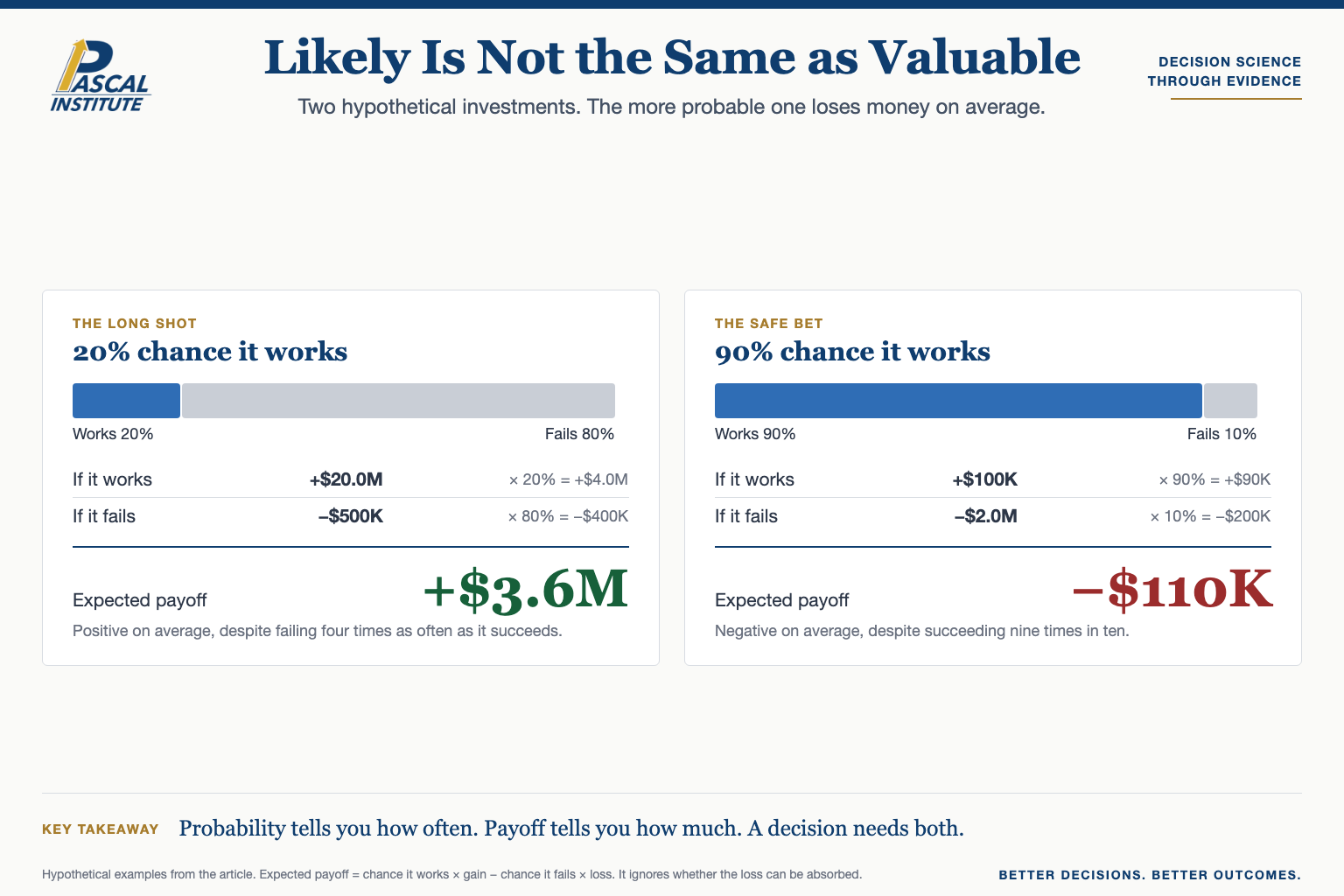
Suppose a hypothetical investment has an 80 percent probability of losing $500,000 and a 20 percent probability of producing a $20 million net gain. Its expected net payoff is $3.6 million, even though failure is four times as likely as success. The investor must still be able to absorb the loss, trust the probability estimates and compare alternatives. Conversely, a venture with a 90 percent probability of producing a $100,000 gain and a 10 percent probability of losing $2 million has a negative expected payoff of $110,000. The higher-probability choice is not automatically the better one.

Finding the Decision Boundary

The practical challenge for managers is deciding how much information is enough. Every forecast contains uncertainty, and every model depends on assumptions that can be wrong. If an organization waits until uncertainty disappears, many opportunities will expire. Decision Science asks how much an estimate would have to change before another alternative becomes preferable.

Suppose a company considers a product expansion with an estimated 70 percent probability of success. After accounting for the value of success, cost of failure and next-best alternative, management determines that the project becomes worthwhile only above 68 percent. A small error could reverse the choice, so additional research may be valuable. If the break-even threshold is 30 percent, the same 70 percent estimate supports a much more robust decision. Knowing whether the true probability is 66 or 74 percent may not change the action.

Houston’s second fourth-and-one resembled the latter case. The modeled conversion probability was far above the estimated break-even threshold. The earlier fourth-and-one was closer: its central break-even estimate was 52 percent, but 95 percent of 200 model refits put the threshold between approximately 29 and 69 percent.⁸ The first decision warranted greater caution than the second, even though the estimated conversion probabilities were similar.

Our initial analysis appeared to show that field position explained much of the difference. Further validation showed that the apparent field-position and clock effects depended on the order in which those variables were changed. The score remained the consistent factor. Moving from a tie game to trailing by seven lowered the modeled break-even threshold by roughly 25 percentage points because the value of a successful field goal changed.⁸

This distinction has consequences for allocating analytical resources. Organizations often spend time improving forecasts by a few percentage points without asking whether those improvements would affect a decision. Moving a forecast from 71 to 73 percent may be statistically useful but operationally irrelevant when the threshold is 30 percent. Improving a forecast from 69 to 71 percent could matter enormously when the boundary is 70 percent. The value of information depends on whether it can change what we choose.

From Analysis to Accountability

A useful Decision Science process begins before committing to an action. Define the objective and possible outcomes. What does success accomplish, and what does failure cost? Identify the alternatives, including waiting when it is genuinely available. Estimate the probabilities using current evidence, then calculate where the preferred choice changes. Test which assumptions matter most and how far they can move before the decision reverses.

At some point, analysis must become action. If the alternatives remain close and information is available at reasonable cost, obtaining it may be worthwhile. If reasonable assumptions consistently favor the same alternative, uncertainty alone is not a reason to avoid choosing. Management should make the decision the evidence supports and record the reasoning before the outcome is known.

That record creates a foundation for accountability. Document the alternatives, probabilities, expected consequences, assumptions and conditions under which the choice would change. When the outcome arrives, compare it with the original forecast rather than reconstructing the reasoning from memory. Successful outcomes can conceal poor decisions just as failures can discredit good ones.¹¹ A well-supported 70 percent project can fail without proving that management was wrong to launch it, and a poorly evaluated acquisition can succeed without proving the process was sound.

The objective is not to excuse failure but to investigate it more accurately. Was the probability estimate poorly calibrated? Did management overlook an alternative? Were the consequences understated? Did information emerge that could not reasonably have been known beforehand? A decision record makes those questions answerable and gives the next team a better starting point.

Over repeated decisions, the record becomes even more useful. Projects assigned probabilities near 70 percent should succeed roughly seven times out of ten when evaluated over sufficiently many comparable cases. If they succeed much less often, the organization has evidence that its forecasting process needs adjustment. If forecasts are calibrated but decisions consistently destroy value, the problem may lie in how the organization prices outcomes or compares alternatives. These are different failures, and they require different remedies.

Houston eventually lost to Cincinnati, and Fairbairn’s attempt came up short. Neither outcome is the reason the evidence favored going for it. Even a successful field goal would have left Houston behind and still needing a touchdown, while the fourth-and-one offered a more valuable alternative. Fairbairn’s previous make was useful evidence about his ability, but it was not evidence that the two opportunities carried the same value.

The purpose of forecasting is to help us understand what might happen. The purpose of Decision Science is to help us determine what those outcomes are worth, compare the alternatives, decide when the evidence is sufficient to act, and learn from the result.